Lighting uniformity in architecture has been a topic of interest for at least seventy years (e.g., IES 1947), where the goal is to encompass the range of illuminance values measured at an array of positions on a horizontal plane, all in a single metric.
 Lighting Uniformity in Horticulture
Ian Ashdown, Senior Scientist and Marc Descoteaux, Senior Software Engineer, | SunTracker Technologies Ltd.
Written in 2015, “Greenhouse Design and Control” (Ponce et al. 2015) is extraordinarily comprehensive in its coverage of greenhouse design issues, from site selection through structural load bearing analysis and ventilation technologies to greenhouse automation using adaptive neural fuzzy inference systems. On the topic of greenhouse lighting, however, it has only this to say: “The light level in the greenhouse should be adequate and uniform for crop growth.”
The authors note that quantum (PAR) sensors are commonly used for photosynthetic photon flux density (PPFD) measurements, but give no guidance on how to measure the lighting uniformity in a greenhouse. This topic has been occasionally discussed in the literature (Both et al. 2002, Ciolkosz et al. 2001, Eaton 2021, Ferentinos et al. 2005, Runkle 2017), but only in the context of supplemental lighting using lighting design software intended for architectural applications. The combination of ever-changing daylight and electric lighting has yet to be considered.
None of these discussions however address the central question: what is “lighting uniformity” in horticulture, and how do we measure (or predict) it?
Architectural Lighting
Lighting uniformity in architecture has been a topic of interest for at least seventy years (e.g., IES 1947), where the goal is to encompass the range of illuminance values measured at an array of positions on a horizontal plane, all in a single metric. These metrics include:
- Coefficient of Variation (Armstrong 1990)
- Entropy-based (Mahdavi and Pal 1999)
- Maximum to average
- Maximum to minimum
- Minimum to average (EN 12464-1)
- Minimum to maximum
- Statistical (Mathieu 1989)
- Uniformity Gradient (Houser et al. 2011)
In practice, only the minimum-to-average illuminance metric is recognized as an international standard (EN 12464-1) for interior lighting design. This is sometimes designated as “U1,” while the minimum-to-maximum illuminance metric is designated as “U2.”
To be honest however, uniformity metrics represent a very simplistic approach to architectural lighting design. They make sense when illuminating large flat surfaces outdoors, such as sports fields, parking lots, and roadway interchanges, but for most interior lighting design applications, they provide little useful information.
Horticultural Lighting
Both the U1 and U2 metrics have been proposed for use in horticultural lighting design by a few luminaire manufacturers, where photosynthetic photon flux density (PPFD, measured in μmol/m2-s) replaces illuminance (lux). This again makes sense because with overhead lighting and daylight, the plant canopy can usually be considered as a large flat surface.
The problem however is that while we perceive visible light reflected from surfaces, plants utilize it for their photosynthetic needs. What we might consider to be almost imperceptible differences in illuminance may be significant in terms of photosynthetic activity and hence plant growth and yield.
Commercial growers have for many decades relied on a rule of thumb that a one percent increase in sustained PPFD (and hence Daily Light Integral) results in a one percent increase in plant growth and yield. Marcelis et al. (2006) quantified this assumption by analyzing yield data from some one hundred academic papers and nearly ninety commercial growers, followed by opinion surveys with eighteen growers. Their research results are summarized in Table 1.
| Crop Group | Crop | Yield Difference |
| Soil-grown vegetables | Lettuce | 0.8% |
| Radish | 1.0% | |
| Fruit vegetables | Cucumber | 0.7 – 1.0% |
| Tomato | 0.7 – 1.0% | |
| Sweet pepper | 0.8 – 1.0% | |
| Cut flowers | Rose | 0.8 – 1.0% |
| Chrysanthemum | 0.6% | |
| Bulb flowers | Freesia | 0.25 – 1.25% |
| Lily | 0.25 – 1.25% | |
| Flowering pot plants | Poinsettia | 0.5 – 0.7% |
| Kalanchoe | 0.8 – 1.0% | |
| Non-flowering pot plants | Ficus | 0.65% |
| Dracaena | 0.65% |
The study results are of course more nuanced than this. For example, the yield difference is greater at lower PPFD levels, higher CO2 concentrations, higher ambient temperatures, and leaf area index. As a result, growers may choose higher temperatures and change their plant density and cultivar choice during times of greater DLI or increased supplemental light levels. In other words, light levels are only one component of farm management.
The key point here however is that uniformity matters when it comes to horticultural lighting. For example, the two gray squares shown in Figure 1 may appear to be almost the same shade of gray to us, but for many plants, they represent a ten percent or so difference in photosynthetic activity and hence plant yield.
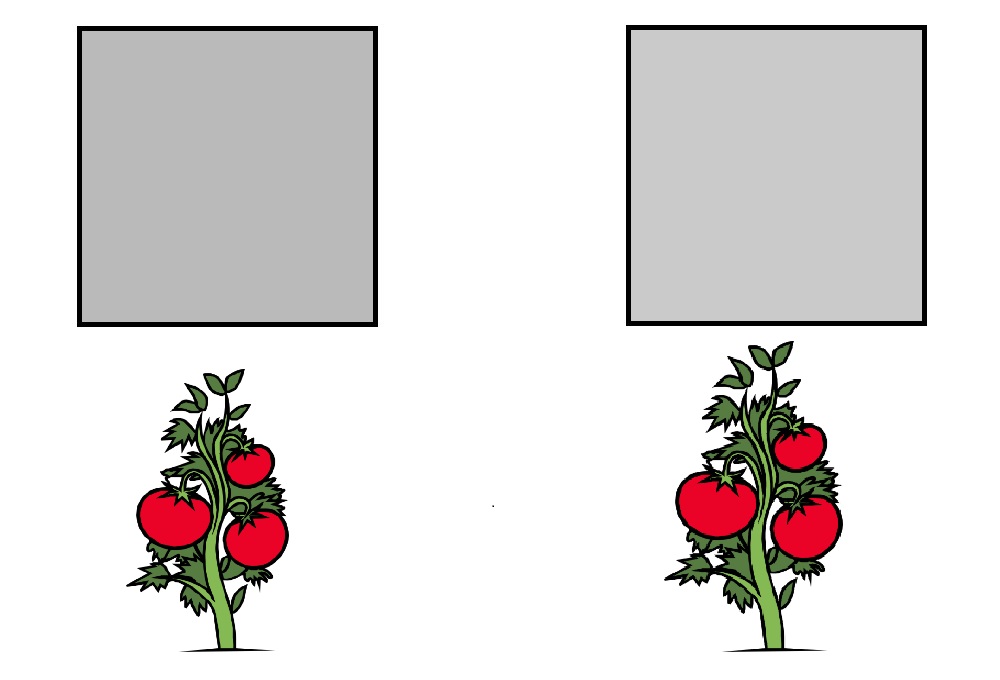
Figure 1 – What we see versus what plants respond to.
Given this, Runkle (2017) has recommended that, “Generally, a 10-20 percent variation in intensity is acceptable.” However, Yelton (2017) and others have proposed that ±5 percent is a more appropriate target for PPFD measurements in greenhouses and plant factories. Figure 1 shows a ten percent difference in plant yield in response to a ten percent increase in PPFD.
Horticultural Uniformity Metric
This suggests yet another uniformity metric, but one that is designed specifically for horticultural lighting. Suppose we are given a virtual model of a small 64×128-foot greenhouse with PPFD values due to electric lighting calculated at two-foot intervals (Figure 2). There are 2048 values, with a maximum of 291.3 μmol/m2-s. The proposed lighting uniformity metric U90 is defined as the percentage of values that are greater than 90 percent of the maximum value, while the proposed lighting uniformity metric U80 is similarly defined as the percentage of values that are greater than 80 percent of the maximum value. (The measurement positions are assumed to be regularly spaced.)
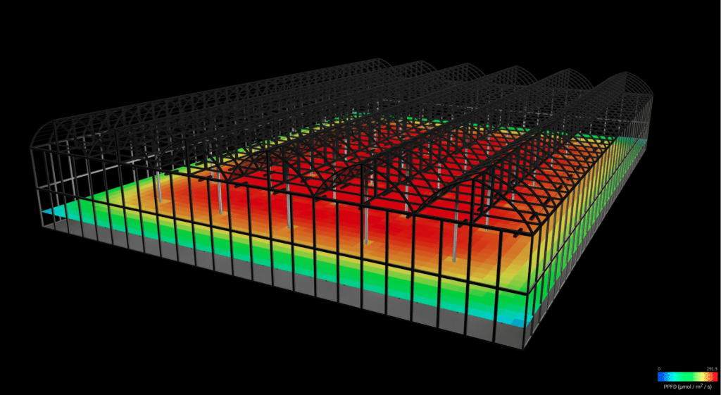
Figure 2 – PPFD distribution in a 64×128-foot greenhouse.
Unlike the architectural U1 and U2 metrics, these two metrics are particularly useful in that they indicate the relative floor area of the greenhouse that is suitable for growing crops. The U90 metric indicates the percentage of illuminated area that satisfies the ±5 percent uniformity requirement, while the U80 metric indicates the percentage of illuminated area that satisfies the ±10 percent uniformity requirement.
Even more useful is that these metrics can be shown in an isoPPFD plot (Figure 3).
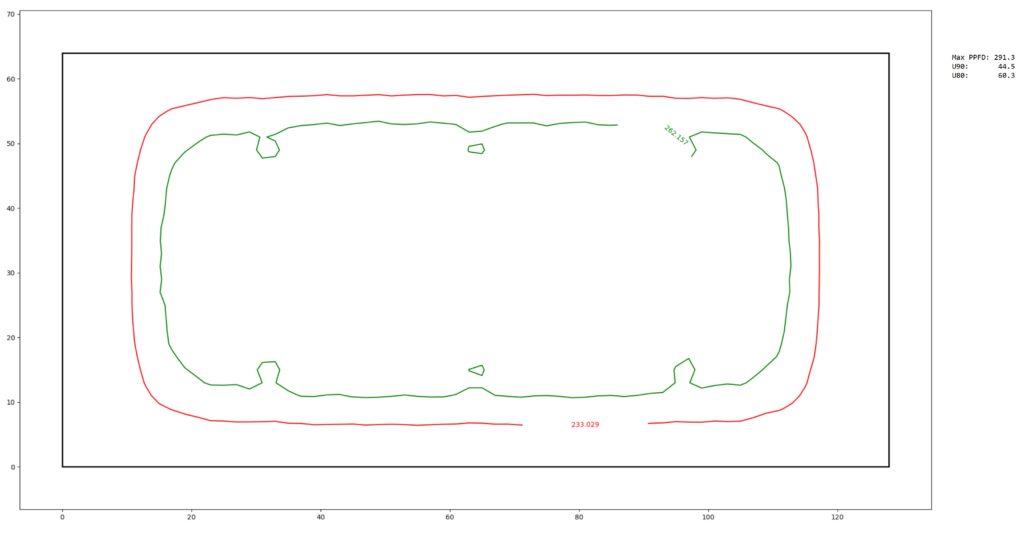
Figure 3 – Small greenhouse isoPPFD plot.
The first reaction will of course be that 44.5 percent usable floor area is terrible in terms of lighting uniformity. This however is precisely the point – the lighting uniformity in a small greenhouse with a regular array of identical luminaires will always be terrible. However, the nonuniformity is due to the area adjacent to the greenhouse walls. Yelton et al. (2017) noted that the uniformity can often be improved by varying the mounting height of the luminaires adjacent to the greenhouse walls, but this may not be an option for practical reasons.
Figure 4 shows a rendering of a commercial greenhouse measuring 512×1024 feet, with 7,680 luminaires, while Figure 5 shows its isoPPFD plot. The U90 metric is 90.0 percent, with the non-uniform areas confined to the floor area adjacent to the greenhouse walls.
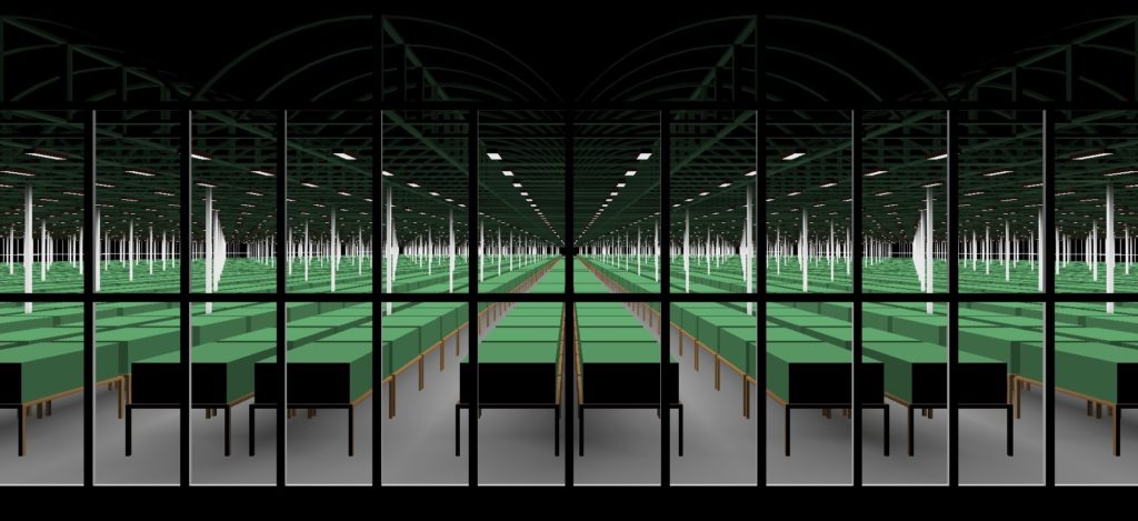
Figure 4 – 512×1024-foot commercial greenhouse.
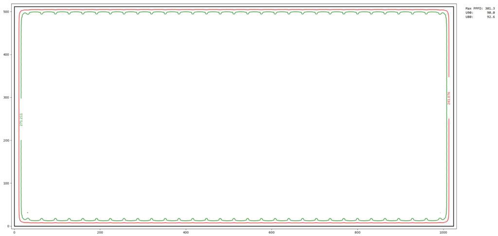
Figure 5 – Commercial greenhouse isoPPFD plot.
The U90 uniformity metric is excellent, but it should be noted that the lighting layout for the commercial greenhouse was chosen to ensure uniformity. Without lighting calculations to validate the uniformity, it cannot be assumed that a given design will satisfy the U90 requirements.
Daylight
We must also remember that the Daily Light Integral (DLI) inside greenhouses is due mainly to daylight, which is much more uniform. Figure 6, for example, shows the monthly average DLI for July with the same greenhouse located in Vancouver, Canada, based on Typical Meteorological Year (TMY3) weather records and solar radiation data from the EUMETSAT weather satellite (Thomas and Ashdown 2022).
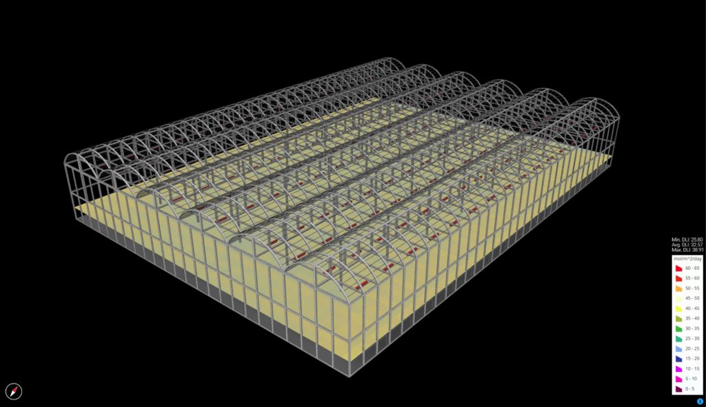
Figure 6 – Monthly average DLI distribution (Vancouver, Canada. July 1970).
Vertical Farms
Where the U80 and U90 metrics become more interesting is in fully-enclosed plant factories, particularly stacked trays in vertical farms. Electrical energy represents between 25 and 35 percent of vertical farm operating costs, and so lighting uniformity for trays is a significant issue.
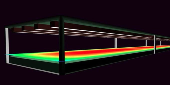
Figure 7 shows three trays measuring 2.1 feet wide by 4.9 feet long, and with a height of 11 inches. The plant canopy height is 1.8 inches. The four rows of luminaires are spaced at 8.0-inch intervals, which appear to provide good uniformity.
Three trays are modeled because, as we saw at the borders of the greenhouse models, we can expect there to be light drop-off at the tray ends.
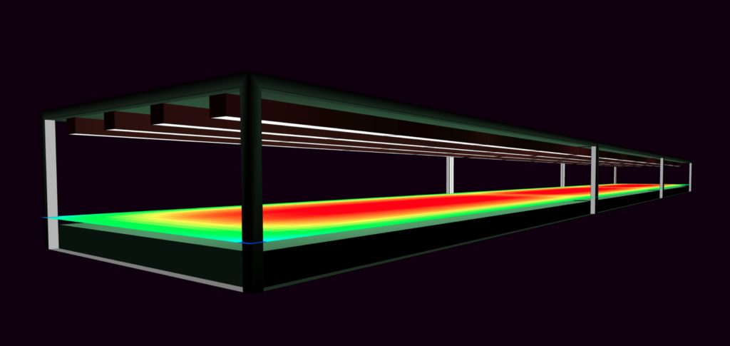
Figure 7 – Vertical farm tray PPFD distribution – canopy height 1.8 inches.
The isoPPFD plot shown in Figure 8, however, shows rather poor uniformity – only 40 percent of the canopy is within the desired ±5 percent uniformity for consistent crop yield.
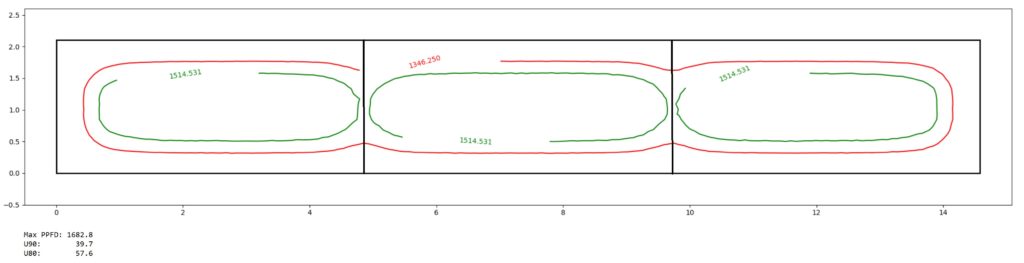
Figure 8 – Vertical farm trays isoPPFD plot – canopy height 1.8 inches.
Equally important is that these results are for plants in the seedling stage. As they mature, the canopy height increases to perhaps four inches or so. As they do, the lighting uniformity will decrease. Figure 9 shows the PPFD distribution for a plant height of 4.2 inches, where the uniformity is obviously less.
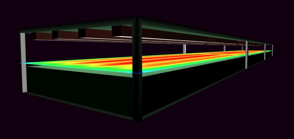
Figure 9 – Vertical farm tray PPFD distribution – canopy height 4.2 inches.
Figure 10 confirms this observation, where the U90 metric is only 21 percent.
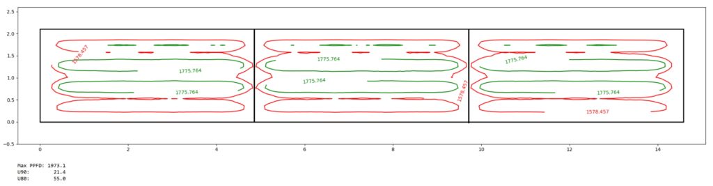
Figure 10 – Vertical farm trays isoPPFD plot – plant height 4.2 inches.
To be fair, the tray height of 11 inches is unusually low. It was chosen specifically to highlight the importance of taking the change in canopy height into consideration when designing tray lighting systems. Greater tray heights will result in improved uniformity, but then reducing the number of luminaire rows for example from four to three will significantly reduce the consistent growing area.
Speaking of tray lighting, there is another issue that uniformity metrics cannot address – spill light. Most horticultural luminaires designed for tray lighting do not include optics to control the beam spread, and so there will be a significant amount of light that ends up on the aisle floor rather than the plant canopy. Properly designed luminaire optics could address this issue to both save electrical energy (and money) and improve lighting uniformity.
Summary
Simply viewing an installed lighting system for a greenhouse or vertical farm will not indicate whether the lighting uniformity is acceptable, and measuring it by hand is a time-consuming and laborious process that may be complicated by the existing infrastructure. It is much better if the uniformity can be calculated during the design stage.
To this end, the U90 and U80 lighting uniformity metrics presented here are specific to horticultural rather than architectural lighting, and along with isoPPFD plots clearly indicate whether the uniformity is acceptable for consistent crop yield.
This report does not consider plant factories with a single layer of plants, such as cannabis production. In this situation, the walls and ceiling should ideally be painted white to maximize reflected light that will improve lighting uniformity. Again however, calculating the light uniformity during the design stage will avoid potential expensive situations once the installation has been completed.
Finally, it should go without saying that accurate predictions of lighting uniformity are only possible with careful measurements of the photosynthetic photon flux intensity (PPI) distributions of the luminiares and careful use of lighting design software to model the application.
Acknowledgements
All greenhouse and vertical farm lighting calculations presented in this report were generated with SunTracker Technologies’ Cerise365+GreenhouseDesigner horticultural lighting design software (www.heliosolsoft.com).
References
- Armstrong, J. D. 1990. “A New Measure of Uniformity for Lighting Installations,” J. Illuminating Engineering Society 19(2):84-89.
- Both, A. J., et al. 2002. “Evaluation of Light Uniformity Underneath Supplemental Lighting Systems,” Acta Horticulturae 580: IV International Symposium on Artificial Lighting. DOI: 10.17660/ActaHortic.2002.580.23.
- CEN. 2002. Light and Lighting – Lighting of Work Places – Part 1: Indoor Work Places, EN 12464-1. European Committee for Standardization.
- Ciolkosz, D. E., et al. 2001. “Selection and Placement of Greenhouse Luminaires for Uniformity,” Applied Engineering in Agriculture 17(6):106-113. DOI: 10.13031/2013.6842.
- Eaton, M. 2021. “Light Simulation in Greenhouses,” GLASE Technical Article Series Issue 8. https://glase.org/technical-articles/light-simulation-in-greenhouses/.
- Ewing, J. L. 1979. “The Price of Uniformity,” J. Illuminating Engineering Society 9(1):47-52.
- Ferentinos, K. P., and L. D. Albright. 2005. “Optimal Design of Plant Lighting Systems by Genetic Algorithms,” Engineering Applications of Artificial Intelligence 18(4):473-484. DOI: 10.1016/j.engappai.2004.11.005.
- Houser, K. W., et al. 2011. “Illuminance Uniformity in Outdoor Sports Lighting,” Leukos 7(4):221-235.
- IES. 1947. IES Lighting Handbook: The Standard Lighting Guide. New York, NY: Illuminating Engineering Society.
- Mahdavi, A., and V. Pal. 1999. “Towards an Entropy-based Light Distribution Uniformity Indicator,” J. Illuminating Engineering Society 28(1):24-29.
- Marcelis, L. F. M, et al. 2006. “Quantification of the Growth Response to Light Quantity in Greenhouse Grown Crops,” Acta Horticulturae 711:97-104.
- Mathieu, J.-P. 1989. “Statistical Uniformity: A New Method of Evaluation,” J. Illuminating Engineering Society 18(2)L 76-80.
- Ngai, P. Y. 2000. “The Relationship between Luminance Uniformity and Brightness Perception,” J. Illuminating Engineering Society 29(1):41-50.
- Ponce, P., et al. 2015. Greenhouse Design and Control, p. 45. Leiden, The Netherlands: CRC Press.
- Runkle, E. 2017. “The Importance of Light Uniformity,” Greenhouse Product News, March, pp. 38.
- Thomas, J., and I. Ashdown. 2022c. “Daily Light Integral Distributions: Geographic Similarity,” ISHS Acta Horticulturae 1337, International Symposium on Light in Horticulture, pp. 265-270
- Yao, Q., et al. 2017. “Evaluation of Several Different Types of Uniformity Metrics and their Correlation with Subjective Perceptions,” Leukos 13(1):33-45.
- Yelton, M., et al. 2017. “Creating Light Uniformity in the Greenhouse,” 2017 ASHS Annual Conference (https://ashs.confex.com/ashs/2017/webprogramarchives/Paper27204.html).
The content & opinions in this article are the author’s and do not necessarily represent the views of AgriTechTomorrow
Comments (0)
This post does not have any comments. Be the first to leave a comment below.
Featured Product